How to Freeze Rows in Google Sheets – Google Sheets Master Guide
Welcome to another exciting Google Sheets tutorial! Have you ever found yourself lost in the vast sea of data in your spreadsheet, desperately scrolling up and down to match column headings with their corresponding rows? We’ve been there too, and that’s why we’re here to unveil the secret weapon: freezing rows.
In this comprehensive guide, we’ll walk you through the ins and outs of how to freeze rows in Google Sheets. But before we dive into the frozen wonderland of data management, if you haven’t yet explored the world of alphabetizing in Google Sheets, we’ve got you covered. Take a moment to check out our previous guide to get up to speed.
Freezing rows is like wielding a digital magic wand in the realm of spreadsheets. It ensures that your crucial data stays put, no matter how far down your spreadsheet journey takes you. Whether you’re a data aficionado or just starting to flex your spreadsheet muscles, let’s embark on this tech-savvy expedition together!
How to Freeze Rows in Google Sheets
Freezing rows in Google Sheets is simple:
- Click on the row number you want to freeze.
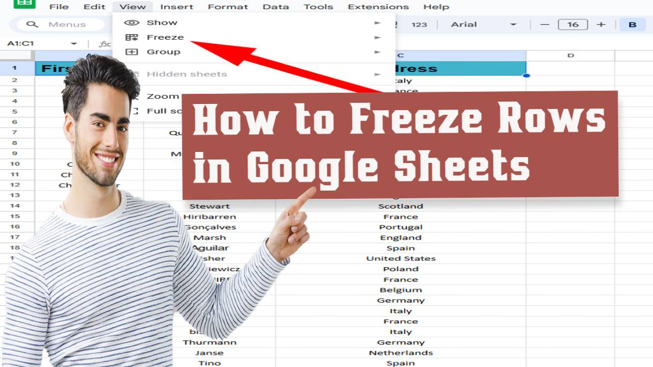
- Go to “View” in the top menu.
- Select “Freeze” and choose “1 row” to freeze top row.
Now, your header row stays visible while you scroll through your spreadsheet, keeping your data organized and accessible.
Why Freeze Rows in Google Sheets?
In the vast landscape of Google Sheets, where data flows endlessly, maintaining clarity and focus can be a challenging endeavor. This is where the magic of freezing rows comes into play. But why is it such a valuable feature?
1.1 Clarity and Consistency
Imagine you’re working on a spreadsheet with numerous columns of data, each containing vital information. As you scroll down, the header row—displaying column titles—vanishes into the abyss, leaving you disoriented. Freezing rows brings consistency to your spreadsheet, ensuring that column titles remain visible, acting as guiding beacons in the sea of data.
1.2 Header Row Perfection
One of the primary use cases for freezing rows is preserving the header row. The header row typically contains essential labels or titles that define the data in each column. Freezing this row means you never lose track of what each column represents, even as you explore thousands of rows below.
1.3 Key Data Always in Sight
In addition to header rows, freezing allows you to keep critical data in view. Let’s say you’re managing a project timeline, and the top rows display important milestones or dates. By freezing these rows, you ensure that these crucial markers are visible at all times, simplifying project management.
1.4 Seamless Navigation
Freezing rows not only enhances data organization but also makes navigation a breeze. Whether you’re analyzing financial data, tracking inventory, or managing schedules, having key information readily accessible as you scroll ensures a seamless user experience.
In essence, freezing rows in Google Sheets is your ticket to a tidier, more organized, and navigable spreadsheet. It’s a feature that transforms chaos into order and empowers you to harness the full potential of your data.
How To Freeze Row In Google Sheets: A Step-by-Step Guide
Freezing rows in Google Sheets is a handy feature that ensures your header row or critical data remains visible as you scroll through your spreadsheet. Here’s how to do it:
Step 1: Select the Row(s) to be Frozen
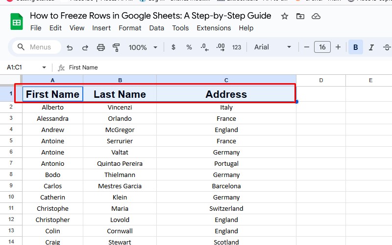
Begin by selecting the row or rows that you want to freeze. This typically includes the header row containing column titles or any other row with essential data you want to keep in view on top.
If you want to freeze only the header than select the header or top row.
In case you want to freeze multiple rows, kindly select all the rows you want to freeze.
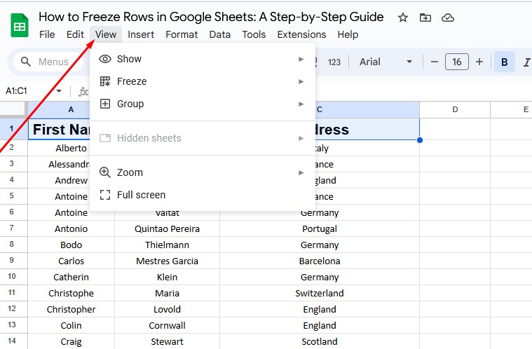
Step 2: Next, navigate to the “View” menu
Next, navigate to the “View” menu located in the top toolbar of your Google Sheets document.
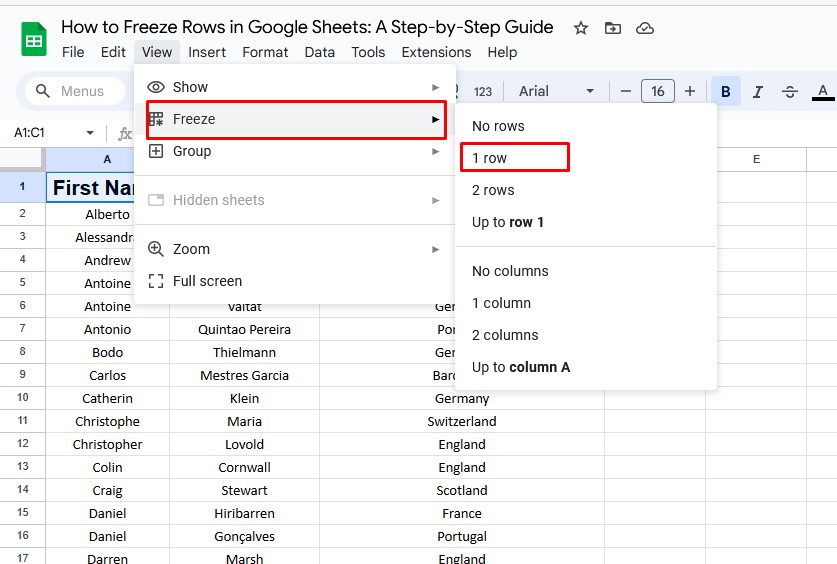
Step 3: Freeze Rows
Within the “View” menu, hover your cursor over the “Freeze” option. A submenu will appear, allowing you to select how many rows you wish to freeze. You can choose to freeze just the top row (usually the header row) by selecting “1 row,” or you can opt to freeze multiple rows if needed.
And that’s it! Your selected row(s) are now frozen, ensuring that they stay visible at the top of your spreadsheet, even as you scroll down to explore your data.
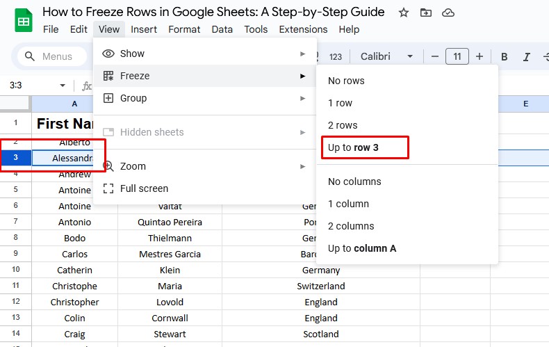
How to Freeze Multiple Rows In Google Sheets
- Click on the row number you want to freeze. For example, if you want to freeze the top three rows, click on the third row number.
- Go to the “View” menu in the top toolbar.
- Select “Freeze” and then choose “Up to row 3.” This option will freeze all rows from the top down to the row you clicked on.
- Now, multiple rows are frozen and will remain visible as you scroll through your spreadsheet.
By following these simple steps, you can maintain clarity and organization in your Google Sheets, making data management a more efficient and seamless process.
Benefits of Freezing Rows
Freezing rows in Google Sheets isn’t just a convenient trick; it’s a game-changer that brings several substantial benefits to your spreadsheet experience.
3.1 Improved Readability in Large Datasets
When working with extensive datasets that span multiple screens, it’s easy to lose context. Freezing rows eliminates this problem by locking specific rows, often the header row, in place. This means that no matter how far you scroll down, you’ll always have a clear view of your column titles. It’s like having a map to guide you through a vast data wilderness.
3.2 Easy Access to Header Information
The header row is the backbone of your spreadsheet. It provides essential information about what each column contains. Freezing this row ensures that this critical information is permanently visible. Whether you’re analyzing sales figures, tracking expenses, or managing a project, easy access to column titles simplifies data interpretation and reduces the risk of errors.
3.3 Enhanced User Experience with Extensive Spreadsheets
Working with extensive spreadsheets can be daunting, especially when you have to scroll endlessly to find specific data points or reference information. Freezing rows transforms this experience into a smooth journey. It keeps vital data at your fingertips, reducing the time you spend searching and scrolling. This not only enhances productivity but also minimizes frustration when dealing with large datasets.
In essence, freezing rows is the secret sauce that enhances the usability of Google Sheets. It’s a tool that improves readability, keeps essential information within reach, and elevates your overall user experience. So, whether you’re managing financial data, organizing inventory, or collaborating on a project, freezing rows is your trusty companion in the world of spreadsheets.
Unfreezing Rows: How to unfreeze rows in Google Sheet
While freezing rows can greatly enhance your Google Sheets experience, there may come a time when you need to unfreeze rows to return to the standard view. Here’s how to do it:
4.1 Unfreezing Rows
Begin by navigating to the row that is currently frozen. This row is typically the top row of your spreadsheet.
Right-click on the frozen row. A context menu will appear.
In the context menu, hover your cursor over the “Freeze” option. A submenu will open.
Within the submenu, select “No rows” or “No rows or columns” to unfreeze the selected row. The option you choose depends on whether you want to unfreeze just the specific row or all frozen rows and columns.
4.2 Reverting the Freezing Effect
If you’ve previously frozen multiple rows or columns and wish to revert the freezing effect, follow these steps:
Click on the “View” menu located in the top toolbar of your Google Sheets document.
In the “View” menu, hover your cursor over the “Freeze” option.
Select “No rows” or “No rows or columns” to unfreeze all previously frozen rows and columns, returning your spreadsheet to its standard view.
Practical Applications
Freezing rows in Google Sheets isn’t just a handy feature; it’s a tool that can significantly enhance various aspects of your spreadsheet work. Here are some practical scenarios where freezing rows proves invaluable:
5.1 Budget Tracking
Managing finances often involves working with large datasets containing income, expenses, and various financial categories. Freezing rows, especially the header row, allows you to keep critical financial categories in view as you scroll through your budget spreadsheet. This makes tracking expenses and maintaining financial clarity a breeze.
5.2 Data Analysis
In data analysis, it’s crucial to have a constant reference point for column titles and data labels. Freezing rows ensures that your headers stay visible, making it easier to interpret data, apply formulas, and generate insights without the risk of losing context.
5.3 Project Management
Project management spreadsheets are notorious for their complexity, with numerous columns and rows tracking tasks, deadlines, and project phases. Freezing rows, particularly the top rows containing project milestones, guarantees that you always have a clear overview of your project’s progress, even as you dive into the details.
5.4 Inventory Management
Whether you’re managing inventory for a small business or tracking items for personal use, freezing rows is a game-changer. It keeps essential information about each item, such as names, quantities, and prices, visible as you navigate through your inventory spreadsheet. This simplifies inventory updates and prevents errors.
5.5 Any Other Relevant Use Cases
The versatility of freezing rows extends to countless other scenarios. Whether you’re creating a schedule, organizing customer data, or collaborating on a team project, freezing rows can streamline your work and boost productivity
Section 6: Additional Tips and Tricks
Freezing rows is just the tip of the iceberg when it comes to optimizing your Google Sheets experience. Here are some additional tips and tricks to consider:
6.1 Freezing Columns
Just as you can freeze rows, you can also freeze columns. To freeze columns, select the column to the left of the one you want to freeze, then follow the same steps as freezing rows. This keeps specific columns visible as you scroll horizontally.
6.2 Freezing Rows on Mobile Devices
If you’re working on Google Sheets using a mobile device, you can still freeze rows for better navigation. Access the “Freeze” option in the mobile app’s settings to keep rows or columns visible on your smaller screen.
6.3 Combining Freezing Rows with Sorting
For advanced data management, consider combining freezing rows with sorting. This allows you to keep your header row in view while sorting data based on specific criteria, making data analysis even more efficient.
Conclusion:
In this comprehensive guide, we’ve explored the power of freezing rows in Google Sheets. We’ve seen how it enhances readability, simplifies data interpretation, and improves overall user experience. Now armed with this knowledge, it’s time to apply these techniques to your own spreadsheet projects.
Remember that freezing rows is not just a feature; it’s a tool that empowers you to conquer the challenges of working with large datasets and complex spreadsheets. So go ahead, freeze rows, unlock the potential of Google Sheets, and make your data-driven tasks smoother and more efficient than ever before.

Hello friends, I am Abhijit, a seasoned virtual assistant and content writer & Co-Founder of getvirtual24.com. Talking about education, I am a History Graduate. I enjoy learning things related to new technology and teaching others. I request you to keep supporting us like this and we will keep providing new information for you.