10 Google Sheets Tips You DON’T Want to Miss 2023

Do you think you’ve mastered Google Sheets?

Think again, buddy.

There’s a whole world of obscure tips and tricks that most people have NO clue about. And learning these hacks is the difference between being a simple spreadsheet amateur and an advanced Google Sheets pro. In case you are just starting out here is our basic guide on How to use Google Sheets.

I’m talking about features so stealthy that barely anyone uses them. Yet they can transform the way you work and analyze data in Sheets.

Don’t believe me? Well in this post, I’m gonna lift the curtain and reveal some of the most useful, hidden secrets in Google Sheets. Ones that will make your other spreadsheet-loving friends jealous once they see the crazy things you can do.

So grab a cup of coffee and get comfortable, my friend. You’re about to go from Google Sheets newbie to certified expert faster than Usain Bolt running the 100 meter dash.

These game-changing tips will unlock the full power of Google Sheets for you. And by the end, you’ll gain superhuman spreadsheet skills and productivity that’ll blow people’s minds.

Jump ahead to any tip by clicking the links above. Let’s dive in and take your Sheets skills up a notch!

1. Scrolling Tables in Google Sheets

Select the data range you want to convert to a scrolling table. Press Ctrl + A to select the entire sheet if needed.

Go to Insert > Chart. This will open the chart creation toolbar.

In the chart type selector, choose the “Table chart” option all the way at the bottom of the dropdown menu

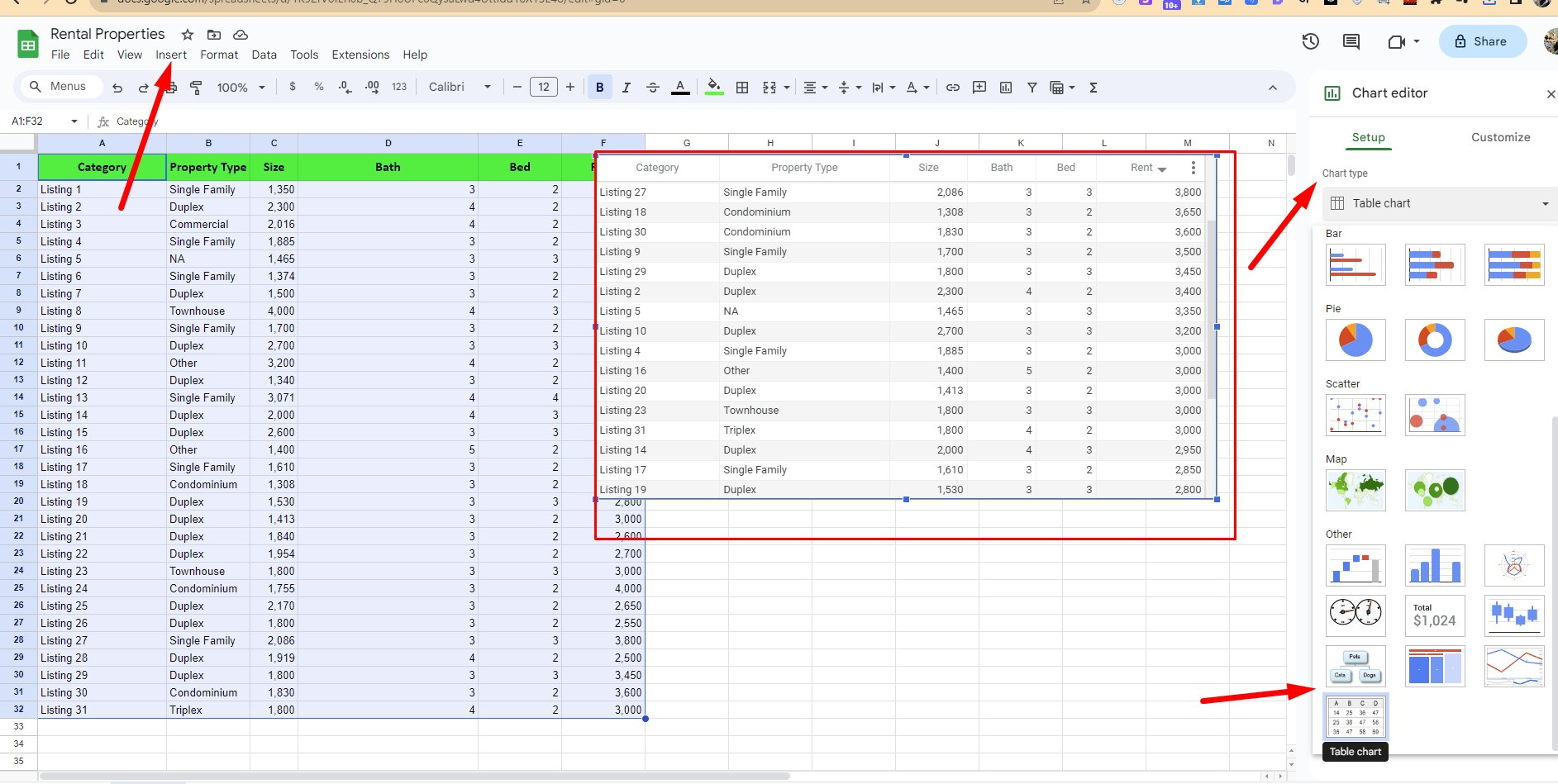
A scrolling table will be automatically created from your data range. You can resize and position the table as needed on your sheet.

The table will include column headings that can be sorted by clicking on them. The sort order will not affect the original data order.

To hide the original data behind the table, cut the data range and paste it onto another sheet

Optionally, add conditional formatting, sparklines, or other customizations to the scrolling table.

The table will stay dynamically connected to the original data source and reflect any changes.

The scrolling table gives you an interactive and organized view of large data sets without cluttering your sheet. Use it for clean, professional data presentation!

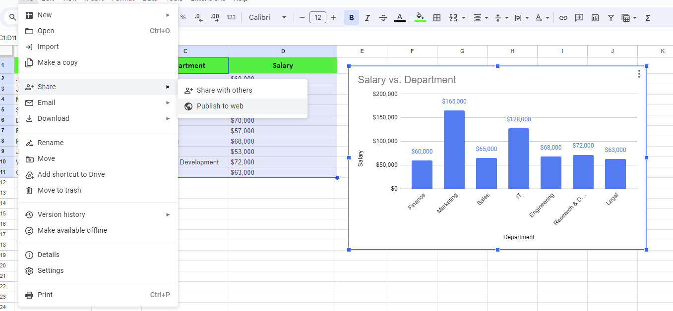
2. Aggregate Chart Values in Google Sheets

Select the data you want to create a chart from, including the column you want to aggregate.

Go to Insert > Chart. Google Sheets will guess the chart type, likely a basic column or line chart.

With your chart selected, open the right side panel. Under the “Aggregate” drop down for the column to aggregate, choose one of the summary options like “Count”, “Sum”, “Average”, etc.

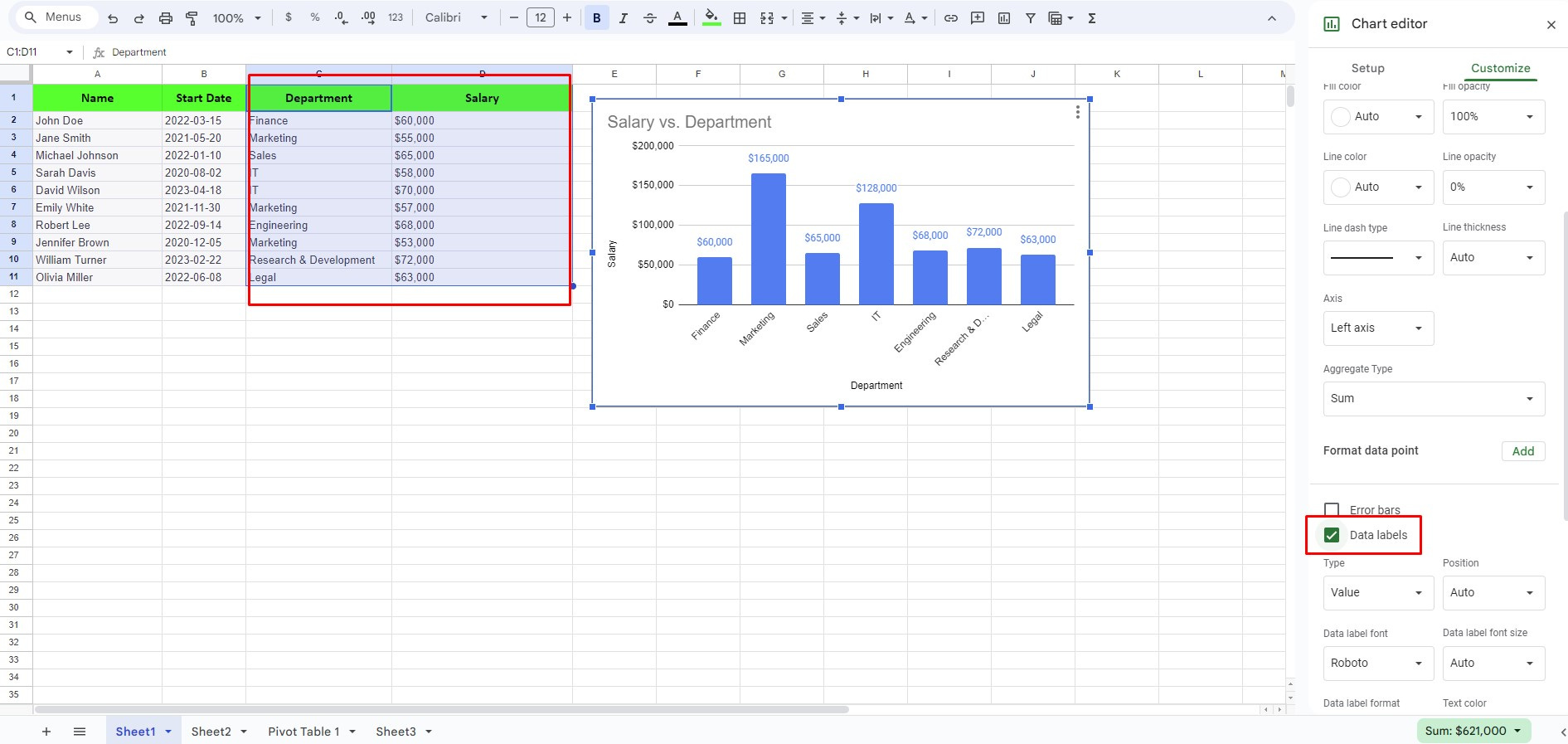
The chart will now display aggregated values rather than individual rows. For example, summing salaries by department instead of each salary.

To add data labels, select the data series and check the “Data labels” box in the Customize tab.

Resize and position your aggregated chart as needed on the sheet.

Adjust the plot area size if needed by dragging the edges to fit titles or labels.

Optionally, add titles, axis labels, additional data series, or other customizations.

The chart will stay dynamically updated if your source data changes.

Aggregating eliminates repetitive values and provides summaries for the big picture view. Use it to simplify complex charts!

3. Publish to the Web in Google Sheets

In Google Sheets, go to File > Share > Publish to web.

In the publish dialog box, choose to publish either the entire document or only a specific sheet.

Click the Publish button.

Copy the published webpage or iframe embed code that is generated.

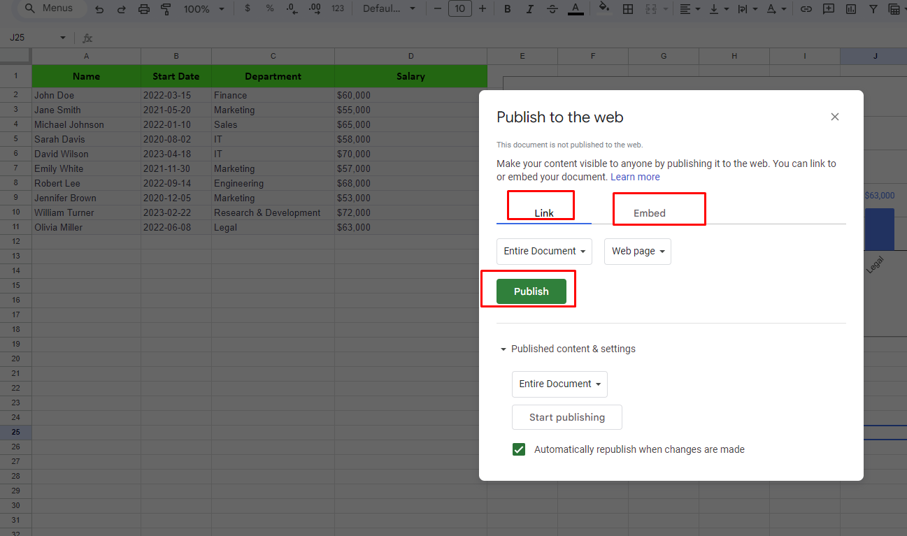
To view the published sheet, paste the web page link into any browser.

To embed the sheet into a webpage, paste the iframe code into the HTML source.

The published sheet will be publicly accessible to anyone with the link. No login required.

Any changes made to the original sheet will automatically sync to the published version.

Use incognito or private browsing to test accessing the sheet when not logged into a Google account.

Share the published sheet link or embed code to distribute the sheet content.

Publishing to the web allows you to easily create live webpages and embed sheets without coding. Great for data dashboards, forms, reports and more!

4. Column Stats in Google Sheets

Column statistics are a great way to get a quick overview of your data without having to create formulas or pivot tables. Let me walk you through how to use them.

First, select the column you want to analyze. You can select just one column, or multiple columns if you want comparative stats. Then, go to the Data menu and click on Column Stats.

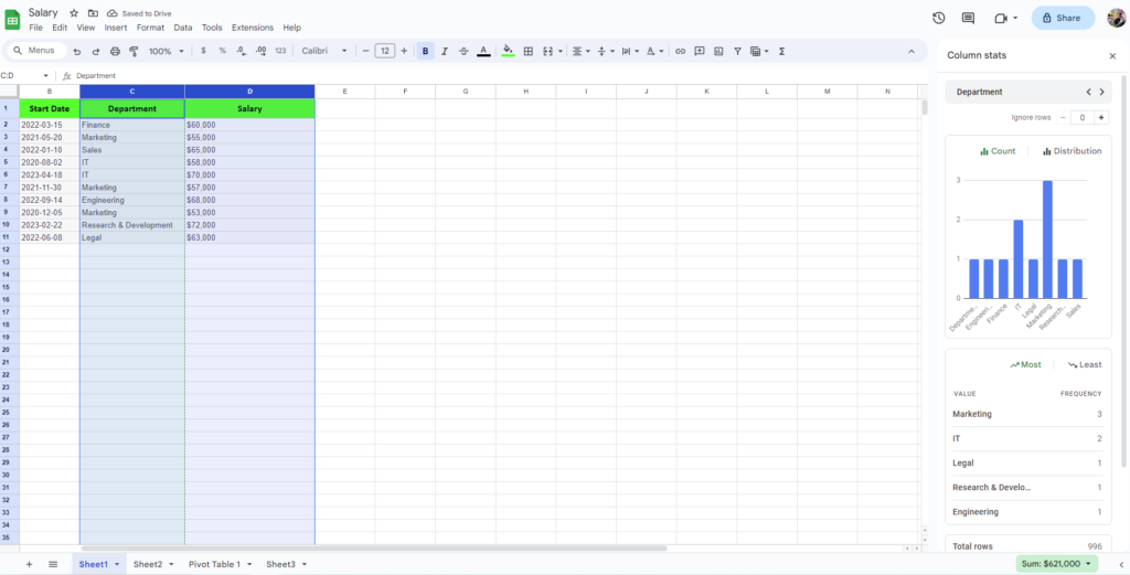
This will open up a panel on the right side of your sheet. Here you’ll immediately get some key figures like the count, mean, median, min and max values. This gives you an idea of total number of data points, average value, minimum value, and Max value.

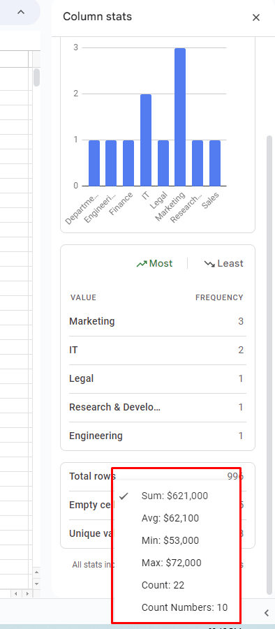
For columns with numeric data, you get a couple additional options. One is quartile values, which show the 25th, 50th, and 75th percentiles. This lets you see how your data is distributed in quarters. There is also an option to change the view to see the distribution as percentages or frequency counts.

Now, one of my favorite parts of column statistics is when you scroll down, you’ll see a full list of each unique value in your selected column along with how often it occurs. This is great for understanding the variability and frequency distribution of your data.

The best part is that all these statistics update automatically if your data changes. You don’t have to re-run formulas or anything. Just refresh the panel. This makes it easy to keep an eye on any changes in the characteristics of your columns.

5. Open-Ended Cell References in Google Sheets

Open-ended cell references are a great trick that allow your formulas to automatically include new data added to a sheet. Let me walk through an example to show you how they work.

Say I have a dataset of sales amounts in column B. I want to calculate the total sales, so I use the SUM formula. Normally, you’d select the cell range to sum, like =SUM(B1:B10). But this is fixed to only sum those specific 10 cells.

With an open-ended reference, we “leave the door open” instead of defining a fixed end. You specify the start of the range, but leave the end of the range blank.

It would look like =SUM(B1:B). This will start summing at cell B1, and keep going down Column B until it hits the last cell with data.

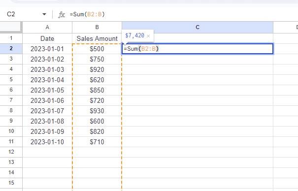
So if I add more sales amounts below the existing data, the total will automatically update. No need to expand the referenced range.

The key is anchoring the start of the range with the $ symbol, like $B$1. This locks it in place. Then leave the end column and row reference blank.

This technique works for many common formulas like COUNTA, MAX, MIN, VLOOKUP, etc. Just remember to lock the start cell, leave the end open.

Open-ended references save you time and ensure your formulas continue working as your data grows. Give them a try the next time you build a spreadsheet! Let me know if you have any other questions.

6. Insert Date From a Calendar in Google Sheets

Adding dates in Sheets can be a pain, but there’s a handy calendar feature that makes it easy. Here’s how to use it:

First, you can enable the calendar picker for any cell by applying data validation. Highlight the cells you want to allow dates in, go to Data > Data Validation, and set the criteria to Date.

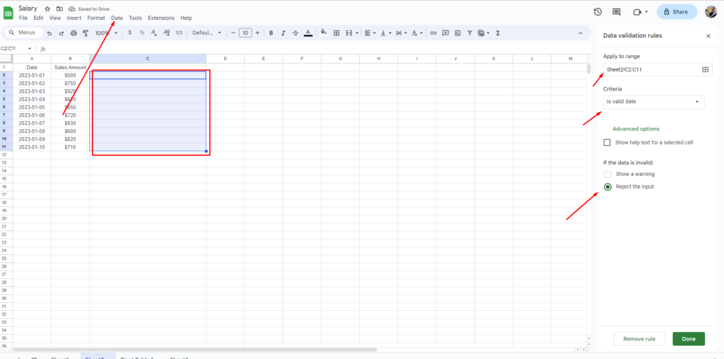
Now when you double click a cell, a little calendar will pop up allowing you to pick the date right from there! Just click the day you want and it will insert it into the cell.

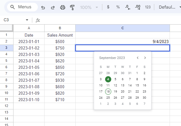
This calendar also has arrows to quickly jump to different months/years. And you can see today’s date highlighted so you can easily choose the current date.

Even better, this calendar picker works inside empty cells too! Normally double clicking an empty cell does nothing.

But with data validation set to Date, the calendar appears right away without having to type anything first. Great timesaver.

To make the dates readable and consistent, be sure to apply a date format like mm/dd/yyyy to those cells after inserting from the calendar.

Using the popup calendar prevents typos and saves you toggling back and forth from the sheet to manually enter dates. Give it a try the next time you need to enter a series of dates!

7. Insert Checkboxes in Google Sheets

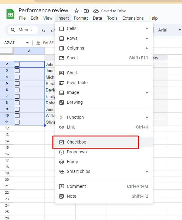
Checkboxes are useful for creating interactive to-do lists, task trackers, forms, and more right in your spreadsheets. Here’s how to add them:

First, highlight the cells you want to place checkboxes inside. Then go to the Insert menu and select Checkbox. This will make checkboxes appear in your selected cells.

By default, the checkbox will be green. To change the color, highlight the checkboxes and update the font color in the toolbar. For example, setting them to orange for visibility.

You can check or uncheck the boxes either by clicking with your mouse, or using the keyboard spacebar. When checked, the cell will show TRUE. Unchecked shows FALSE.

In the formula bar, you’ll see the checkbox has the CHECKBOX function. You can reference these boolean outputs in formulas. Like automatically turning text red if checked.

Checkboxes are interactive, so anyone viewing or editing the sheet can toggle them on and off. Great for lists, project management, data validation, and more.

Give them a try next time you need interactivity in your sheet! Let me know if you have any other questions.

8. Pivot Tables in Google Sheets

Here are the instructions for using Pivot Tables in Google Sheets without numbering or bullet points:

Ensure your data is organized with clear headers and no empty rows or columns.

Select your data by clicking on any cell within your dataset or highlighting the entire dataset.

Go to the “Insert” menu and select “Pivot table.” Google Sheets will identify your data range.

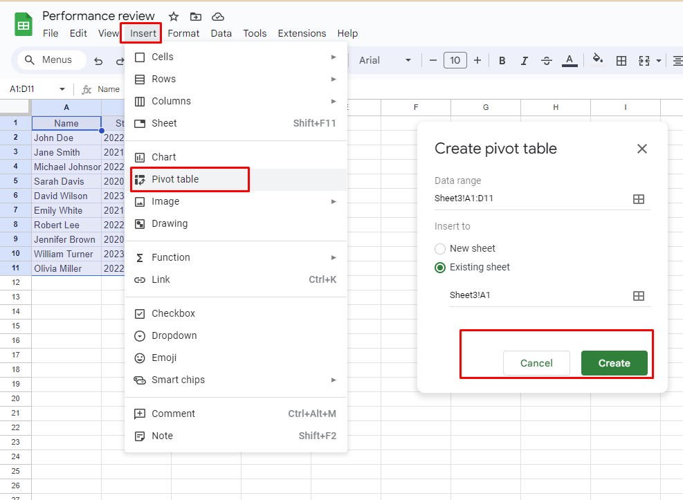
Customize the Pivot Table in the editor:

Drag and drop column headers for row labels (e.g., “Department” for salary data) into the “Rows” section.

Choose column headers for multi-dimensional views in the “Columns” section.

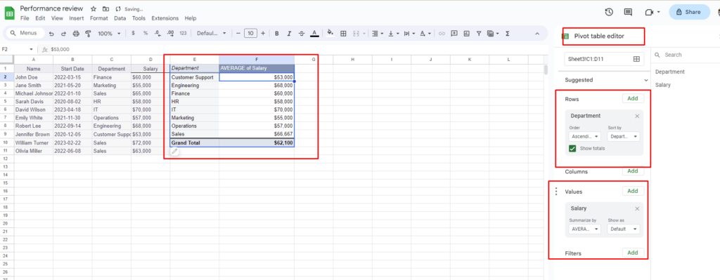
Select numerical data (e.g., Salary amounts) and apply aggregation functions like SUM, AVERAGE, COUNT, etc., in the “Values” section.

Adjust formatting, rename columns, or change aggregation functions as needed.

Double-click on any cell to explore underlying data contributing to a specific value.

If your source data changes, refresh your Pivot Table by clicking inside it and selecting “Refresh.”

Use your Pivot Table to analyze data, create charts, apply filters, and make data-driven decisions.

Pivot Tables in Google Sheets are a versatile tool for data analysis and reporting.

9. How to Use IMPORTHTML in Google Sheets

To use IMPORTHTML in Google Sheets, you can follow these steps:

First, open your Google Sheets document and find the cell where you’d like to import data from a web page.

Next, you’ll need to enter the IMPORTHTML function into that cell. You can simply go to insert > Function > Web > IMPORTHTML.

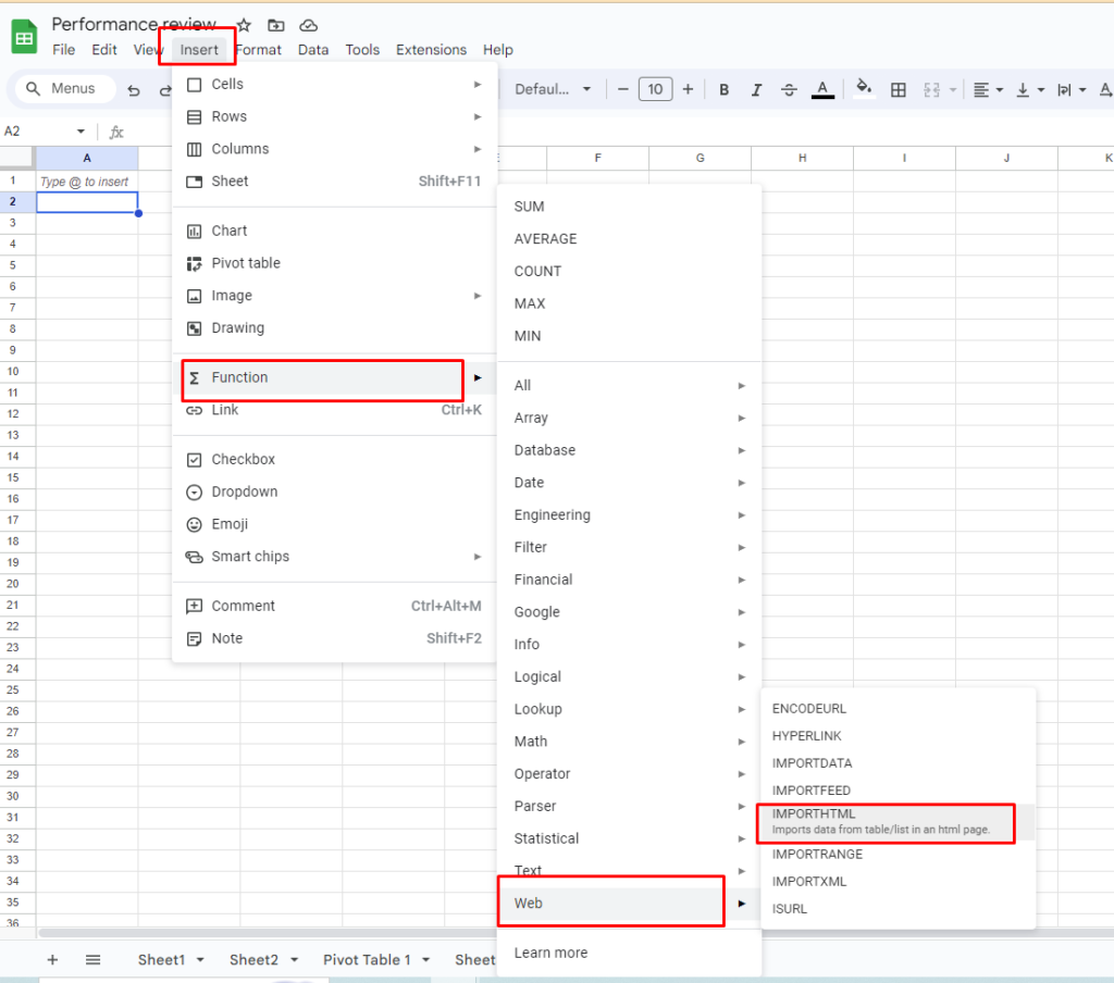
The function has three parts: the web page URL you want to import data from, the type of data you want to extract (like a table, list, or ordered list), and an optional index number if there are multiple tables or lists on the page.

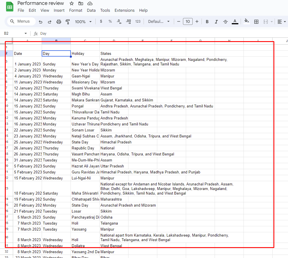
Lets say I want to import “National Holidays in India 2023” from this page – https://www.getvirtual24.com/national-holidays-in-india-2023/

The formula might look something like this: =IMPORTHTML("https://www.getvirtual24.com/national-holidays-in-india-2023/", "table", 1). In this case, we’re importing the first table from “https://www.getvirtual24.com/national-holidays-in-india-2023/“.

After you’ve entered the formula, just press Enter. Google Sheets will fetch the data from the specified web page and display it in your chosen cell.

Remember that the imported data won’t automatically update. If you need the data to refresh, you can manually re-enter the formula or set up automatic updates in your Google Sheets settings.

Lastly, you can also insert screenshots of the web page or the imported data into your spreadsheet if needed. Simply go to “Insert,” choose “Image,” and then select “Image in cell.”

By following these steps, you’ll be able to effectively use IMPORTHTML in Google Sheets to import data from web pages. Make sure to replace the example URL with the actual web page URL you want to pull data from and adjust the parameters as necessary to get the specific information you need.

10. Filter Functions in Google Sheets

The filter functions in Google Sheets are extremely useful for dynamically manipulating your data. Some of my favorites include:

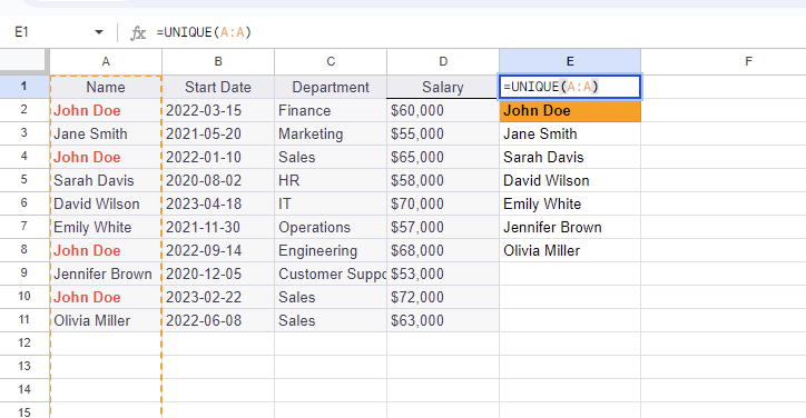
UNIQUE – This returns a list of only the unique values from a range. Great for creating dynamic drop-downs. Just enter =UNIQUE(A:A) for a list of unique values from column A.

SORT – Sort allows you to customize the sort order. For example, =SORT(A2:B, 1, FALSE) will sort your data by Column A, descending.

FILTER – This lets you filter your data based on criteria. Like =FILTER(A:C, B:B=”Complete”) to show rows where Status is Complete.

You can nest these together too. If you do =UNIQUE(FILTER(A:A, A:A<>””)) it will filter blanks, then give unique values.

The key benefit over just using built-in filters is that these formulas dynamically update. So your unique lists, sorts, and filters will recalculate based on the latest data.

I recommend exploring the filter category under Insert > Function to see all the possibilities. Examples include query, pivot table filters, by row/column, and more.

These supercharge your data analysis and allow very customized views. Let me know if you need help implementing any filter formulas!

Conclusion

In this article, we’ve taken a deep dive into ten fantastic Google Sheets tips that can significantly boost your efficiency and productivity when working with spreadsheets. We started by exploring the concept of scrolling tables, which allow you to create interactive tables that are perfect for reports and charts. Then, we delved into auto-aggregating chart values, a feature that simplifies data visualization.

We also discussed how you can publish your Google Sheets online or embed them on websites, making data sharing a breeze. The “Column Stats” feature was another highlight, providing quick insights into your data. Open-ended cell references allow you to future-proof your formulas by dynamically adjusting to new data.

Adding checkboxes to your sheets for to-do lists and task tracking became a straightforward process, and we even looked at pivot tables for dynamic data analysis. Web functions like “IMPORTHTML” enable you to pull data from web pages effortlessly. Finally, we touched upon the versatility of Google Sheets’ functions in organizing and filtering data dynamically.

To further expand your knowledge, we encourage you to explore our comprehensive guide on “How to Use Google Sheets.” With these newfound skills, you’ll be better equipped to harness the full potential of Google Sheets in your daily tasks.

In closing, we’re genuinely excited to assist you in becoming a Google Sheets pro. With these tips in your toolkit, you’ll find that managing and analyzing data becomes more efficient and enjoyable. Your success is our priority, so please feel free to reach out with any questions or feedback. Happy spreadsheeting!